Stress Distribution of Soil (Layered Soil Medium)- Part 04

Stress distribution through layered soil mediums

Burmister developed the chart given below to estimate the vertical stress distribution through a two layer medium. the chart is developed to estimate the vertical stress below the center lines of a circular loaded area and the thickness of a layer 1 is assumed ti be equal to the radius of the circular loaded area.





where,
v = poisson's ratio
E = young's modulus

The stiffness ratio between the two layers in the governing factor ( E1 / E2) in determining the stress distribution among layers.

Examle :
A 2 m diameter foundation is resting on a 2 layer medium having top layer thickness of 1 m. layer 1 has as elastic modulus of 50000 K Pa and layer 2 has an elastic modulus of 5000 K Pa. both layers have the poisson's ration as 0.5 estimate the stress increment 2 m below the center line of the loaded area. (q = 100 K Pa)


E1 / E2 = 50000 / 5000 = 10
Z/b = 2/1 = 2   (b = radius)
by graph,
sigma z / q = 0.17
but q = 100
therefore,
sigma z / 100 = 0.17
sigma z = 17 K Pa

The stress distribution given by the chart for the two layer system is of particular importance in foundation engineering, where shallow foundations are constructed in hard stiff filled layers, which overlies soft compressible layers.

In such situations, it is seen from the chart below that the stress applied on the bottom layer significantly reduced if the stiffness ration is high.

In highway engineering, the road subgrade and the pavement are of significantly different stiffness and hence, the assumption of homogeneous medium is not applicable.

Osterburg Method (for embankments) 

In influence diagram for the vertical stress at any depth Z directly beneath the vertical edge of the semi-embankment can be estimated by using the chart proposed by Osterburg.

 
where,
sigma c = stress
I = influence value (by graph)
q0 (max stress) = unit weight of the embankment material x Height of the embankment = gamma x H

Procedure of the Osterburg method

Chart have 2 parameters,

1) B1/Z and B2/Z using that we need to find influence factor Iz.

2) Then apply to the equation
qv = Iz q0
where,
q0 = gamma soil x H

B1 = 0 , B2 = 0 possible

Example :

Stress at point B

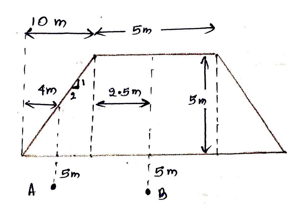
 gamma = 20 K N/m^3

B1 = 2.5 , B2 = 10

therefore,
B1/Z = 2.5/5 = 0.5
 B2/Z = 10/5 = 2
from chart I2 = 0.44

q0 = 20 x 5 = 100 K Pa

Stress a point B = [0.44 x 100] x 2 = 88 K Pa

Note: need to multiply by 2 because there are 2 sections, if sections are not identical we need to calculate for that and need to add

Stress at point A

section X

B1 = 11 m, B2 = 10m

B1/Z = 11/5 = 2.2
B2/Z = 10/5 = 2

q0 = 20 x 5 = 100 K Pa
Iz = 0.49

therefore X, qx = 0.49 x 100 = 49 K Pa

section Y

B1 = 0, B2 = 4
B1/Z = 0
B2/Z = 4/5 = 0.8

q0 = 20 x 2 = 40 K Pa
Iz = 0.2

for Y, qy = 0.2 x 40 = 8 K Pa
  
section Z

 B1 = 0, B2 = 6
B1/Z = 0
B2/Z = 6/5 = 1.2

q0 = 3 x 20 = 60 K Pa
Iz = 0.26

section Z ; qz = - 0.26 x 60 = - 1536 K Pa

Total stress at A = 49 + 8 - 15.6 = 41.4 K Pa

Example :
Estimate the vertical stress increment at point A and B due to the weight of the embankment. (unit weight of material is 20 KN / m^3)